PRINCIPAL COMPONENT ANALYSIS
METHOD 2: PRINCIPAL COMPONENT ANALYSIS


PRINCIPAL COMPONENT ANALYSIS:
So, first, let's look at what it truly means:
Principal Component Analysis is a well-known linear dimensionality reduction approach. This strategy directs the data to a lower-dimensional space while maximising the variance of the data in the low-dimensional representation.
Trust me, if you are finding this confusing means you’re definitely getting it :)
Talking about Linear transformation approach:
Converts a series of possibly correlated observations into a set of linearly uncorrelated 'variables' values (principal components)
Explains a big portion of data variance with a small number of primary components.
NOTE: We will generally use the term “variables” and “features” to denote the independent features in the original dataset and “dimensions” to denote those obtained from these variables by PCA.
HOW, WHY, AND EVERYTHING IN BETWEEN PCA AND MATHEMATICS:

Before you scroll down for the sake of maths. Don't worry, I've attempted to make arithmetic less terrifying for you. I promise, just try to remember one thing: simply comprehend the notion of how things operate and let models handle the arithmetic! (For the time being, just suppose that we are only getting the concept of why we are performing arithmetic rather than really doing maths.)
STANDARD DEVIATION
Try to analyse the below image once:

The standard deviation can be plotted in the Excel graph and is known as the "bell-shaped curve." (as you see above)
Placing a bell-shaped graph depicts the highest chance of the event, and as the bell shapes travel to either side of the centre point, the likelihood of the occurrence decreases.
The bell curve will be put on the right-hand side of the bell curve in the higher range, the left-hand side of the bell curve in the lower range, and the middle of the bell curve in the average range.
Let us begin with the most basic definition, which simply states that:
The standard deviation is a number that reflects how evenly distributed the values are.
Lowering the standard deviation means that the majority of the statistics are close to the mean (average).
Higher standard deviation indicates that the data are spread out across a larger range.
FORMULA:

NOTATIONS:
σ = Popular Standard Deviation
xi = Terms Given in the Data
μ = Population Mean
N = Size of the Population
ROLE OF STANDARD DEVIATION IN PCA?
The Standard Deviation (SD) of a data collection is a measure of how spread out the data is. Assists us in standardising the data, which is the first and most significant stage in principal component analysis. It calculates the data's variability.
2. VARIANCE:
Variance relates to how the model evolves when various parts of the training data set are used. Simply putting, variance is the variability in model prediction—how much the ML function may change based on the data set.
In layman's terms, variance indicates how far a random variable deviates from its expected value.
FORMULA:

NOTATIONS:
S² = Sample Variance
xi = The value of the one observation.
x̄ = The value of the one observation.
n = The number of observations
ROLE OF VARIANCE IN PCA?
The variance of a dataset is a statistical measure of how much variation can be linked to each of the principles.
COVARIANCE:
The covariance matrix is a p * p symmetric matrix (where p is the dimension number) that contains the covariances associated with all possible pairings of the starting variables as entries.
Covariance is a measure of how much each dimension differs from the mean in relation to each other.
Covariance is calculated between two dimensions to determine whether there is a link between the two dimensions.
NOTE: The variance is the correlation between one dimension and itself.
This much covariance is enough to understand the upcoming steps but if you wanna dig deep into COVARIANCE please visit this bomb article by:
https://towardsdatascience.com/5-things-you-should-know-about-covariance-26b12a0516f1
FORMULA:

NOTATIONS:
cov_{x,y} = covariance between variable x and y
xi = data value of x
yi = data value of y
x̄ = mean of x
ȳ = mean of y
N = number of data values.
ROLE OF COVARIANCE IN PCA?
They calculate the variance of individual random variables and determine if variables are linked.
The higher this value, the more dependent the connection is. A positive value represents positive covariance, which suggests a direct link. A negative value, on the other hand, signifies negative covariance, which indicates that the two variables have an inverse connection.
EIGENVECTORS AND EIGENVALUES:
The eigenvectors and eigenvalues of a covariance (or correlation) matrix represent the “core” of a PCA:
The eigenvectors (principal components) determine the directions of the new feature space, whereas the eigenvalues determine their magnitude.
FORMULA:
EIGENVECTOR:
Ax = λx
EIGENVALUE:
A - λI = 0
Remember that an eigenvalue λ and an eigenvector x for a square matrix A satisfy the equation Ax = λx. We solve det(A - λI) = 0 for λ to find the eigenvalues. Then we solve (A - λI)x=0 for x to find the eigenvectors
(I represents the Identity matrix)
NOTE: For a n-dimensional square matrix, there are at most ‘n’ no. of eigen-vectors and ‘n’ no of eigen-values.
SUMMARY:
Eigenvectors are the Principal component directions
Eigenvalues are the magnitude of stretch
Eigenvalues represent the magnitude of variance along those directions.
ROLE OF EIGENVECTORS AND EIGENVALUES IN PCA?
Eigenvalues are just the coefficients associated to eigenvectors that provide the magnitude of the axis. They are the measure of the data's covariance in this circumstance. You may acquire the principal components in order of importance by ordering your eigenvectors in order of their eigenvalues, highest to lowest.
BUT FIRST, BEFORE PERFORMING THE PCA:
Let's check the box of requirements we just completed before constructing and working with the real data set.

Understanding the concept behind DATA DIMENSIONALITY REDUCTION ✅
Got familiar with CURSE OF DIMENSIONALITY ✅
Got Introduce to PRINCIPAL COMPONENT ANALYSIS ✅
Shook hands with MATHS used for PCA ✅
Well equipped with Standard Deviation ✅
Variance is Information, YEAH remembered that ✅
Understood everything about Covariance ✅
Eigenvalues and eigenvectors done as well ✅
Let's combine all of the aforementioned ideas and break them down into a step-by-step procedure for computing the PCA:
STEP1: GETTING THE DATASET TO WORK WITH:

STEP2: STANDARDIZATION:
This step's goal is to normalise the range of continuous baseline variables such that they all contribute equally to the analysis.
Assume we have two variables in our data collection, one with values ranging from 1-100 and the other with values ranging from 100-1000. The output calculated with these predictor variables will now be skewed since the variable with a broader range will have a more evident influence on the outcome.
FORMULA FOR STANDARDIZATION:
Z = value - Mean / Standard Deviation
STEP3: CALCULATING COVARIANCE MATRIX:
The goal of this stage is to understand how the variables in the input data set differ from the mean in relation to each other, or to discover whether there is any link between them. Because variables are often so closely connected that they contain duplicate information. So, to find these connections, we construct the covariance matrix.
Consider the following scenario: we have a 2-dimensional data set with variables ‘a’ and ‘b’, and the covariance matrix is a 2*2 matrix:

In the preceding matrix:
Cov(a, a) reflects a variable's covariance with itself, which is just the variance of the variable 'a.'
Cov(a, b) denotes the covariance of variable a with respect to variable b.
Cov(a, b) = Cov(a, b) since covariance is commutative (b, a)
STEP4: CALCULATING THE EIGENVECTORS AND EIGENVALUES :
Eigenvectors and eigenvalues are linear algebra concepts that must be computed from the covariance matrix in order to discover the principal components of the data.
PRINCIPAL COMPONENTS ?
Simply explained, primary components are the new collection of variables created by subtracting the initial set of variables. The principal components are estimated such that newly obtained variables are highly significant and independent of one another. The main components condense and include the majority of the important information that was dispersed across the original variables.
If your data set has 3 dimensions, then 3 principal components are computed, with the first principal component storing the most possible information and the second storing the remaining maximum information, and so on.
WHERE DO EIGENVECTORS FIT INTO ALL OF THIS?
Assuming a three-dimensional data collection with three eigenvectors (and their corresponding eigenvalues) calculated. The aim behind eigenvectors is to utilise the Covariance matrix to figure out where the most variance exists in the data. Eigenvectors are used to identify and compute Principal Components since higher variation in the data signifies more information about the data.
Eigenvalues, on the other hand, are just the scalars of the eigenvectors. As a result, the Principal Components of the data set will be computed using eigenvectors and eigenvalues.

DON'T WORRY; ONCE YOU START DOING THE PRACTICAL CODE FILE AHEAD, ALL OF THIS THEORY WILL BE CRYSTAL CLEAR.
STEP5: REDUCING THE DIMENSIONS OF THE DATA SET

Apart from standardisation, no changes are made to the data in the preceding phases; you just choose the primary components and build the feature vector, but the input data set is always in terms of the original axes (i.e, in terms of the initial variables).
The goal of this final step is to reorient the data from the original axis to the ones indicated by the main components using the feature vector created by the eigenvectors of the covariance matrix ALSO TERMED AS PRINCIPAL COMPONENT ANALYSIS. This could be accomplished by multiplying the original data set's transpose by the feature vector's transpose.
MATHEMATICAL FORMULA FOR THE ABOVE THEORY:
FinalDataSet = FeatureVectorT * StandarizedOriginalDataSetT
TIME FOR MY MOST - FAVOURITE PART

LET'S GET STARTED ON WITH THE PRACTICAL:
Before I begin, I feel that language 'R' is the easiest of all, thus my code file is written in that language. But, if Python is your real passion, I've attached a reference from one of my favourite (i.e codebasics) that will help you put all of the above theory into practise and make things easy and comprehensible.
Reference for PYTHON:
CODEBASICS CODE FILE (LANGUAGE = PYTHON) (Incase you prefer Python over R)
WRITTEN BY DSMCS:❤️
CHECK OUT THE CODE FILE (LANGUAGE =R): where I tried to apply all of the above approaches and worked with real data to see how things end up in PCA.
CHECKOUT THE FINAL RESULTS AND DO LET US KNOW WHAT DID YOUFIND AND LEARN!💙INCASE, YOU ARE STRUGGLING WITH DATASETFEEL FREE TO MAIL US AND WE WOULD BE MORE THEN HAPPY TO HELP!❤️MAIL-ID: VIDHIWAGHELA60@GMAIL.COMFOLLOW US FOR UPCOMING CODE FILES on DATA DIMENSION REDUCTION SERIES:GITHUB: https://github.com/Vidhi1290/DSMCS/blob/main/PCA.ipynbINSTAGRAM: https://www.instagram.com/datasciencemeetscybersecurity/?hl=enLINKEDLN: https://www.linkedin.com/company/dsmcs/MEDIUM: https://medium.com/@datasciencemeetscybersecurity/method-2-principal-component-analysis-30236d86df30- Team Data Science Meets Cyber Security ❤️💙


Comments
Post a Comment